Bootstrapping an Analytics Environment Using Open Source & Google Cloud Platform

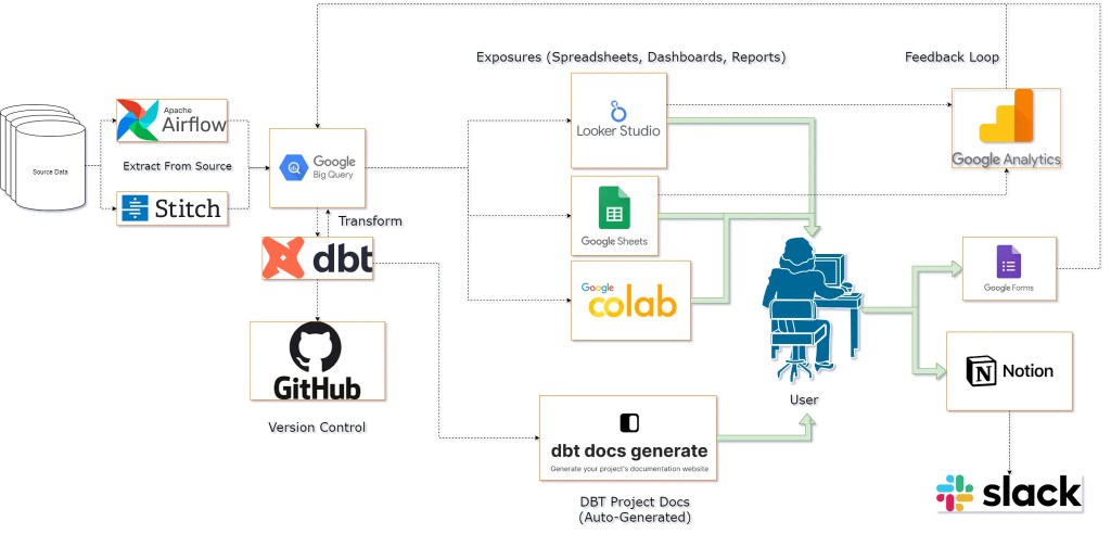
When I first started working at my job, there was a need for an analytics data warehouse where analysts can pull clean & trusted data without having the dreadful task of always searching, asking and validating for nearly every data request. There were a few different projects working separately all generating data in various locations, and was difficult at times to pull things together. A previous analyst named Alex had started this initiative & coined the name for our pipeline the “Analytics Pipeline”, and thus it was named.

This is a proprietary project so I’m going to withhold things like schema names and actual code. I will try to capture the project at a high-level as it takes place over an entire year.

Data Build Tool or DBT is really the magic sauce here. It’s open source & very powerful. I’ve used or tested every feature in DBT’s offering, and I love the tool. I am not going to mention or list all features in this project, only the core ones that I use regularly.

Extracting & Loading Data

Because DBT can only transform our data, we will do that last. Historically we’ve called this “ETL” which stands for Extract, Transform, Load. In modern times, compute and storage are cheaper than before so we can just copy the source data into our target system, then transform it in the same environment.

Airflow & GCP, Stitch Data

Airflow is another open source tool used for CI/CD. There are several legacy processes that run here and is leveraged by the Analytics Pipeline. No additional work was needed, just worth mentioning.

Stitch Data is a paid service that also came with a few legacy processes. Stitch is a great tool based on which sources it has access to, and its ease of use. Fun fact however, Stitch Data is just a wrapper for https://www.singer.io/, another open source tool meant for simply extracting data from source systems into a database.

BigQuery

BigQuery is part of the Google Cloud Platform environment, and is the system we already use so we will continue to do so. Its cheap, fast & integrates pretty much automatically as we’re “google” people.

Data Transformation With DBT

---

I love DBT, love that it’s open source & love what I can accomplish with it. This tool is ideal for people who write lots of SQL code. With DBT you can really automate lots of the boring and tedious, hard to maintain code behind data warehouses. It also brings improvements to the analytics workflow if you’re into building well-defined KPI’s, Metrics or SQL Models. Every table, column, description, relationship, metric, report, dashboard, notebook all in one place, and version controlled (meaning you can “go back” to old versions, and see whether your change will break anything, before committing to it). Ultimately, if you’re someone working in a data warehouse, responsible for writing SQL & you need a better system, look into using DBT to organize, build & test your data warehouse.

I’ve used DBT extensively in this project, pretty much covering everything that DBT has to offer. I’m going to try and focus on the core stuff in here, so I’ll be skipping things like Docs, Tests, Semantic Models, Metrics and Jinja-Macros. The core of DBT are sources, models, .yaml files (how to use them), and lineage.

High Level DBT Object Lineage

Configuring DBT involves only 2 files: a data_model.sql & a data_model.yml file.

The .SQL file contains the SQL code your database will read.

The .YML file contains the metadata. You SQL model is likely a tabular/denormalized model. The .YML contains things like the table name, descriptions, data types, column names and descriptions, tests, and other possible configurations.

In my implementation, I opted for the Source -> Staging -> Intermediate -> Data Marts structure.

Here’s a real-world example using some Shopify data sourced indirectly from their API.

Building a Shopify Data Pipeline with Metrics & an Automated Dashboard

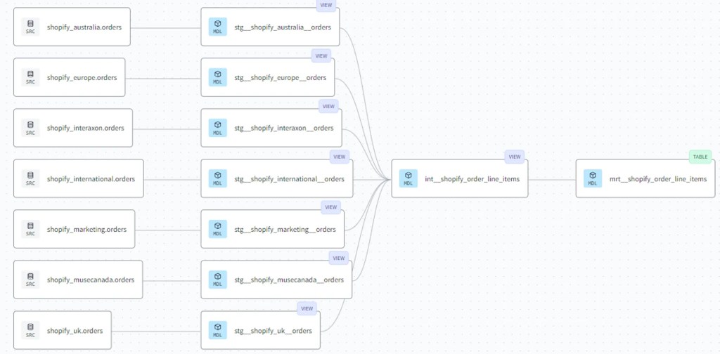
In this database, there were multiple Shopify stores due to tax considerations. Which leaves us with a copy of source data for each store, and no easy way to query all the stores together.

The following will be my implementation of modelling this data by combining it and cleaning everything up. The main thing I strive for with a big table like this is to capture the lowest grain, in our case this data contains order line-items, which allows us to see the financial data per line item which will always be useful for product analytics.

Source Layer

The source layer in DBT is simple a .yml file explaining what table in the warehouse is the source table. In our case, this is our Shopify Orders table for each region.

1. Definitions are stored in the big doc block. I’ve written them once, and use them for each Shopify source. They are kind of confusing so just know its a way to share definitions across objects, and I’ve not totally figured out the most elegant system yet so its kind of hard to maintain. Needless to say, below is an example .yml file for the first few columns in the shopify_europe source.

# .YML FILE
sources:
- database: my-database-id
  description: '{{ doc("shopify") }}' # A common definition for each shopify store, stored in Doc Block
  name: shopify_europe
  tables:
  - columns:
    - data_type: string
      description: '{{ doc("shopify__orders__customer_locale") }}'
      name: customer_locale
    - data_type: record
      description: '{{ doc("shopify__orders__billing_address") }}'
      name: billing_address
    - data_type: int64
      description: '{{ doc("shopify__orders__user_id") }}'
      name: user_id
    - data_type: numeric
      description: '{{ doc("shopify__orders__total_price_usd") }}'
      name: total_price_usd
      # ... rest of the columns

Staging Layer

This layer is meant to be as close to the source as possible. We need a way to quickly reference the source, and select everything from a table. All columns are specified and these files can be automatically created. One gotcha here is that if the column is a record, object, json, etc. data type, it will not be “unnested”. Because of these, you need to still “go in” and unpack these objects, where necessary (such as in this case for Shopify Orders).

# .SQL FILE
{{ config(materialized='view') }}

with source as (

    select * from {{ source('shopify_europe', 'orders') }}

),

renamed as (

    select
        customer_locale,
        billing_address,
        user_id,
        total_price_usd,
				-- .... rest of the columns

    from source

)

select * from renamed

Intermediate Layer

The model here is doing a few things.

1. Creating an event-based table from the “orders” object. Orders have refunds, returns, and purchases. These are represented as properties (columns) of the order objects (rows) but I need them (columns) to be events (rows).
   • This is an example of how the data is structured in the source layer

order	order_date	refund date
order_1	yyyy-mm-dd	yyyy-mm-dd
order_2	yyyy-mm-dd

• Now here’s an example of of the data is structured after the “int” transformation is applied:

order	event type	date	amount
order_1	purchase	yyyy-mm-dd	1
order_1	refund	yyyy-mm-dd	-1
order_3	purchase	yyyy-mm-dd	1

2. The script also loops through each store, and applies the same transformation to each store, using the name as a variable. This is an example of using Jinja in our SQL.

# .SQL FILE
{{ config(materialized='view') }}

with orders as (

-- START LOOP --> 'shopify_stores' is defined in dbt_project.yml
{% for (store) in var('shopify_stores') %}
  
  select distinct
    name                                                                                                                  as order_number,
    datetime(o.created_at, 'America/Toronto')                                                                             as event_datetime_toronto,
    'Purchase'                                                                                                            as order_event,
    -- .... REST OF THE COLUMNS
    '{{store}}' as shopify_store_source
  from {{ ref('stg__' + store + '__orders') }} o
  left join unnest(line_items) li
  left join unnest(shipping_lines) sl
  where true  
    and financial_status in ('paid')

  union all --------------------------------------------------------------------------------

  select distinct
    name                                                                                                                  as order_number,
    datetime(r.value.processed_at, 'America/Toronto')                                                                     as event_datetime_toronto,
    'Refund'                                                                                                              as order_event,
	   -- .... REST OF THE COLUMNS
    '{{store}}' as shopify_store_source
  from {{ ref('stg__' + store + '__orders') }} o
  left join unnest(line_items) li
  left join unnest(shipping_lines) sl
  left join unnest(refunds) r
  left join unnest(r.value.refund_line_items) rli
  where true
    and financial_status like 'refunded'




  /*Now dealing with the partial refunds. 
  These happen as order credits, and not at line-item level. */ 
  union all---------------------------------------------------------------------------------

  select distinct
    name                                                                                                                  as order_number,
    datetime(r.value.processed_at, 'America/Toronto')                                                                     as event_datetime_toronto,
    'Partial Refund'                                                                                                      as order_event,
    -- .... REST OF THE COLUMS
    '{{store}}' as shopify_store_source
  from {{ ref('stg__' + store + '__orders') }} o
  left join unnest(line_items) li
  left join unnest(shipping_lines) sl
  left join unnest(refunds) r
  left join unnest(r.value.order_adjustments) as roa
  where true
    and financial_status like 'partially_refunded'
    
{% if not loop.last %}
    UNION ALL
{% endif %}
{% endfor %}

),

final as (
    select * from orders
)

select * from final

Mart Layer

The “final” model layer, meant for use in production. This layer has no rules, but I try to be efficient. Everything that didn’t make sense to add in the previous layer goes in here. In our case, we’re adding some USD exchange rate data to help match our financial reporting. This was done after the first round of validation with stakeholders as I learned that they had specific requirements for reporting in USD, opposed to base currencies from each of the Shopify stores.

# .SQL FILE
{{ config(materialized='table')}}

with

src_shopify_order_line_items as (
  select * from {{  ref('int__shopify_order_line_items')  }}
),

src_usd_exchange_rates as (
    select * from {{ ref('int__sales_copy_na1__fx_rates') }}
),

adding_exchange_rate_logic as (
    select 
        s.* except(usd_exchange_rate, total_price_usd, revenue_usd, order_status, shopify_store_source),
    case 
        -- if morning exchange time is closer to event date, then morning rate. Else end of day rate
        when abs(date_diff(datetime(r.morning), datetime(event_datetime_toronto), hour)) >= abs(date_diff(datetime(r.end_of_day), datetime(event_datetime_toronto), hour))
            then r.morning_rate
            else r.end_of_day_rate
        end as usd_exchange_rate,
        replace(initcap(order_status),'_',' ') as order_status,
        replace(initcap(shopify_store_source),'_',' ') as shopify_store_source,
    from src_shopify_order_line_items s
    left join src_usd_exchange_rates r on date(r.fx_dates) = date(event_datetime_toronto) and lower(r.base_currency_code) = lower(s.presentment_currency)
),

adding_columns as (
    select 
        *,
        round(usd_exchange_rate * revenue_base, 2) as revenue_usd,
    from adding_exchange_rate_logic
),

final as (
  select * from adding_columns
)

select * from final  
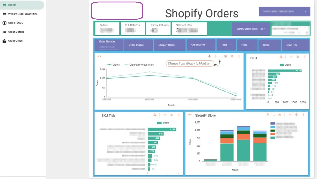
where date(event_datetime_toronto) < current_date() -- this helps as our exchange rate data is not yet updated same-day

Exposures (Reports & Dashboards)

Exposures are used here to track which reports use which data marts and are super simple to setup. Its basically just the metadata, with a link to the report. Here is an example:

# .YML FILE
version: 2

exposures:

  - name: shopify_orders
    label: Shopify Orders Dashboard - Purchase, Refund, Partials in $USD
    type: dashboard
    maturity: high
    url: https://bi.tool/dashboards/1
    description: >
      Did someone say "exponential growth"?

    depends_on:
      - ref('mrt__shopify_order_line_items')

    owner:
      name: First Last
      email: name@email.com

Version Control, CI/CD & Documentation

---

GitHub & DBT Cloud

For this project we’re using DBT Cloud (paid service) and GitHub (free) to drive our CI\CD (continuous integration and continuous delivery/deployment). DBT Cloud runs on a set schedule, and during this run will incrementally refresh the latest data into the table. It will always use the latest version on the main branch in GitHub, so any changes that were committed since the last run will automatically be picked up & integrated.

Exposures & Feedback Loop

---

The top 3 exposure types are Google Sheets for quick analysis, Looker Studio for more concrete & automated reporting, as well as Google Colab for bringing your data into a Python environment, key for any analyst or scientist. We support all of these sources with direct connection to the Analytics Pipeline through various types of security measures. The feedback loop comes into play here as it’s right where the user is, using the data with their data tools!

Google Analytics is used to track web traffic events, and we use this to track usage to key Google Sheets & all Looker Studio dashboards. Google Colab is a little more tricky, so it does not get the same treatment. It also gets far less traffic, so we don’t have a strong use case to track it yet.

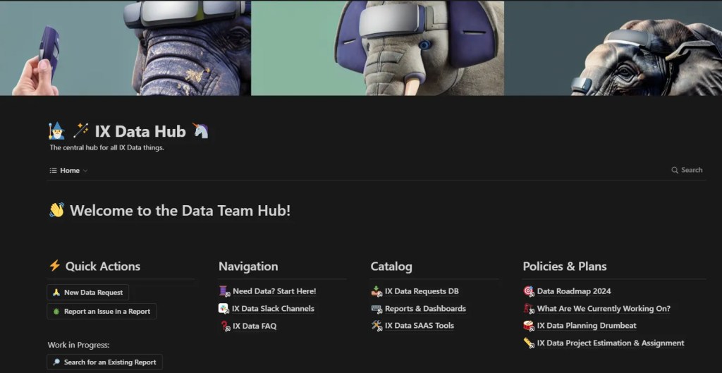
Google Forms are a handy tool for quickly adding user feedback on a dashboard by adding a link to a feedback form right into the report. I’ll briefly mention Notion as well, as we use it to capture inbound requests related to dashboards. We like Notion because of the built in Slack integration, so when someone requests something we all get a ping to let everyone know instantly.

Scaling Challenges & Roadmap Problems

---

In no particular order, the following things are pain points, even with all the automation we have today.

1. Data Governance, PII & PHI
   1. How do we enforce rules, save time, grant access, track usage – safely, quietly and within regulatory compliance standards?
2. Documentation strategies
   1. How do we build a habit/culture of including documentation into our projects?
   2. How do we ensure documentation isn’t a waste of time? Make sure its useable by everyone, forever?
3. Scaling the team
   1. How do we name, commit, change, review, document our work?
   2. What are the housekeeping tasks that need to be done?
   3. What should be automated vs could be?

Conclusion

The Analytics Pipeline demonstrates the benefits of well-implemented data engineering practices. By utilizing tools like DBT, Airflow, Stitch Data, and BigQuery, this system streamlines the process of managing complex data, transforming scattered datasets into a unified and automated analytics solution.

Each component of the pipeline plays a crucial role – ensuring data quality, enabling transformations, and facilitating insightful analytics that drive better business decisions. This meticulous approach improves operational efficiency and unlocks the true value of data-driven intelligence.

While challenges lie ahead, the future of the Analytics Pipeline looks promising. Strengthening data governance, expanding documentation efforts, and growing the team strategically will reinforce the foundations built by this pioneering project. Continuously gathering feedback, integrating user input through tools like Google Forms and Notion, and maintaining a strong focus on security and compliance will ensure the pipeline remains relevant and adaptable.

In short, The Analytics Pipeline exemplifies the power of innovation, collaboration, and commitment to data excellence. As this system evolves, it serves as a model for others in the industry, proving that with the right tools, strategies, and mindset, complex data can be transformed into clear, actionable insights that drive business success.